
Log in to the site
SDM (species distribution modelling) is an ecological modelling method that predicts the geographic distribution of different species of animals, plants and fungi.
Qb.SDM is a software package implementing SDM algorithms.
The Qb.SDM user interface runs in the browser and is available at https://wingeds.world/sdm
This document contains the documentation for the Qb.SDM software package, together with a general description of SDM algorithms.
1. SDM: modelling species distributions.
1.1. Description of the SDM approach.
1.2. Limitations of SDM as a method.
1.3. Fields of application of SDM and examples.
1.4. Overview of methods that extend or relate to SDM.
2. Qb.SDM: information about the software package.
2.2. Qb.SDM: description of input parameters.
2.3. Qb.SDM: presenting and interpreting results.
2.3.1. The “modelling results” section.
2.3.2. The “quality metrics” section.
2.3.3. The “response curves” section.
2.3.4. The “predictor importance” section.
2.4. Qb.SDM: technical description of the algorithms:
2.4.1. Observation pre-processing.
2.4.2. Predictor pre-processing.
2.4.3. Preparing background points and pseudo-absence points.
2.4.4. Accounting for species mobility (the M-factor).
2.4.5. Description of how the model works.
SDM is an ecological modelling method that predicts the geographic distribution of species. Alternative names for the method: ENM (ecological niche modelling), BEM (bioclimatic envelope modelling), HOM (habitat occupancy modelling), SIP (species invasions projections) [1].
The source data for SDM are:
- observations - information about the species' presence (geographic coordinates);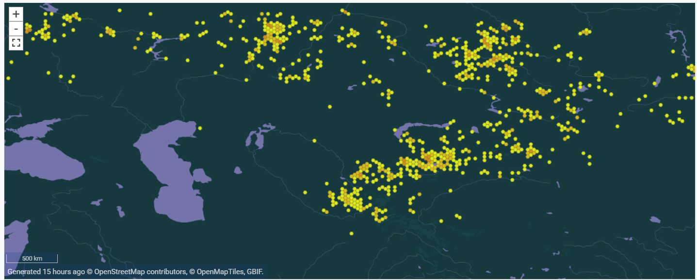
Predictors, i.e. biogeographic variables, are a set of maps containing values that characterize the modelling region. Examples: mean annual temperature and its amplitude, total precipitation and mean annual humidity, elevation and slope, physical and chemical soil composition, etc.
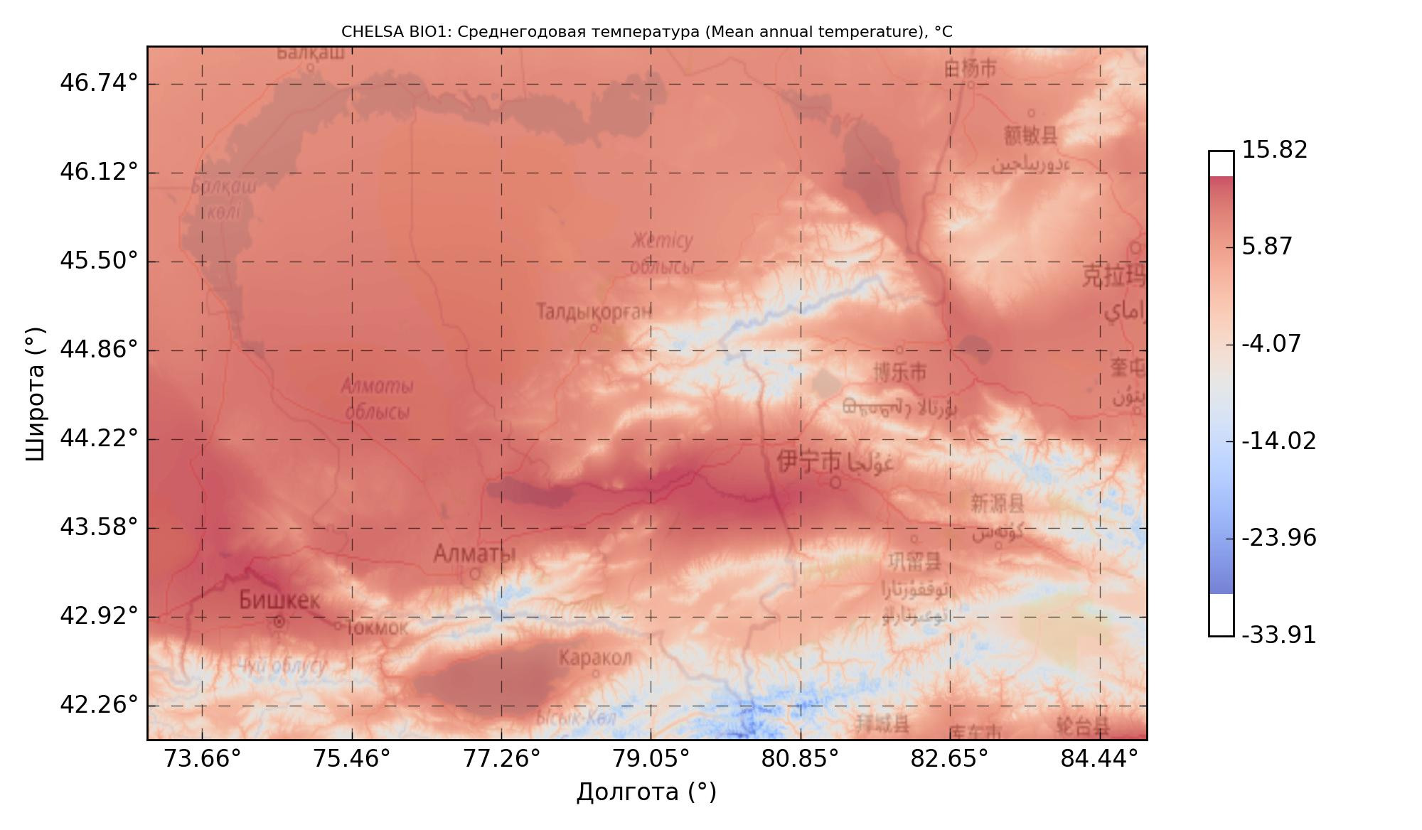
This data is fed into an algorithm (one of several machine-learning methods: Random Forest, XGBoost, MaxEnt, etc).
The algorithm finds the relationship between observations and predictors, i.e. the conditions suitable for the species. The algorithm's output is usually described as the probability of the species' presence at a given point (strictly speaking, from an ecological standpoint it is more correct to speak of habitat suitability at that point for the species). The model's output is a value from 0 to 1, often expressed as a percentage from 0% to 100%.
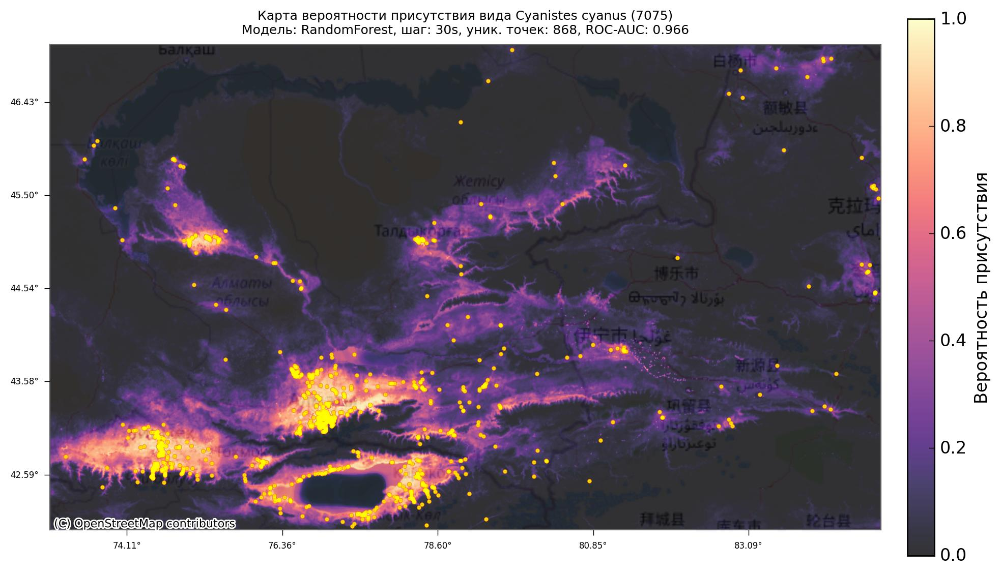
The algorithm is then applied to every geographic point within the specified region, computing the probability of presence (habitat suitability) for each one. For visualization, the result is projected onto a geographic map:
The core idea of SDM is to identify the “comfortable conditions” for a species. By comfortable conditions we mean a set of climatic and other parameters under which the species can persist over the long term (habitat).
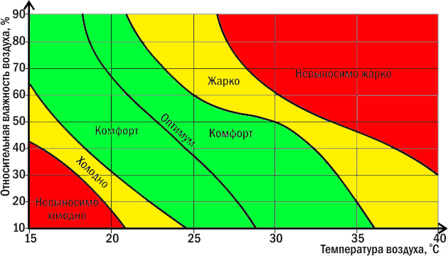
Ecological niche (following G.E. Hutchinson) is the functional place of a species within an ecosystem, encompassing the entire set of its requirements for living conditions (habitat: temperature, humidity, etc.) and its role in the biocenosis (biotic factors: trophic relationships, competition, etc.).
SDM is built on the niche conservatism hypothesis. This is the assumption that different individuals of a species occupy the same ecological niche, and that this ecological niche does not change over the period being modelled by SDM - or that any such change is small enough, relative to the modelling range, to be neglected.
The output of SDM is the search for suitable habitat for a species. SDM is often said to model a species' ecological niche - however, in the strict ecological sense this is not accurate, since SDM typically does not model biotic factors. [1]
The mechanics of SDM work as follows:
1) The collected observations are projected onto the predictor-layer maps:
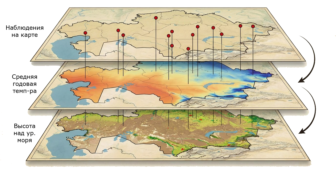
2) The projection yields an array of bioclimatic-variable values at the species' observation points:

3) Based on this array, the conditions (set of variables) under which the species can exist are computed. These conditions are taken to be the ecological niche within the space of the given predictors.
Note that this is not the entire ecological niche, since these conditions do not account for biotic interactions:
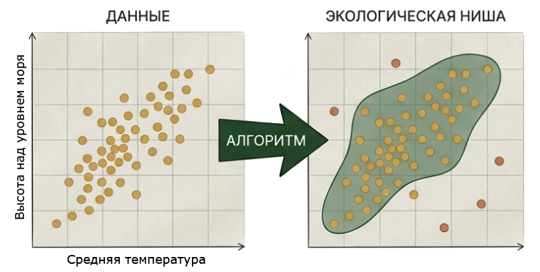
Outside the observation points, background points and pseudo-absence points are generated. Background points are distributed uniformly at random across the available area. Pseudo-absence points are generated using the RSEB algorithm: at a certain distance from the species' occurrence points. For more on the RSEB method, see section 2.4.3 and [3].
4) For presence points the target variable is set to 1; for background points and pseudo-absence points the target variable is set to 0.
5) A machine-learning algorithm is then run on this dataset. During training, a regression problem is solved: for any given set of bioclimatic variables, the model produces a prediction in the range from 0 to 1 - the degree of habitat suitability.
6) For every point on the map, the corresponding set of bioclimatic-variable values is determined. The model is applied to them, and the result is then projected onto the map.
The output of SDM is presented in the form of a map.
Visualization options:
- presence-probability values;
- or a threshold value is set (for example, 95%), and the map marks all areas with a probability value above that threshold. To visually highlight such areas, an enveloping “buffer” of several kilometres is often added (for example, 1-5 km).
1.2. Limitations of SDM as a method.It is important to understand exactly what SDM models: suitable habitat.
That is, areas where the bioclimatic variables match the conditions required for the species to exist (according to the model).
Traditional SDM does not account for the following factors:
- biotic factors (competition, trophic relationships, etc.); - historical factors (for example, the species' past distribution may have been limited by an ice age); - geographic factors (for example, the species cannot cross a mountain range or a body of water); - factors that were not explicitly fed into the model (for example, the species may require a specific soil salinity, but no such predictor was used for training); - seasonality and migration.However, there are many extensions of SDM that add consideration of these factors. For more detail see section 1.4. Some of these factors are also modelled in Qb.SDM
Thus, SDM may show areas where the species is not currently present, but where suitable conditions exist (according to the model, given the predictors used). Alternatively, the species may simply not have been observed there (no observers) - and such areas may be worth investigating more closely.
The reverse situation is also possible, where the species is present in areas not indicated by the model. Possible reasons:
- an observation made outside suitable habitat, for example during migration, while fleeing a predator, etc.; - the model is not accurate enough (for example, it does not account for predictors that affect this species); - some factor in that area has a positive effect on the species even outside its comfortable habitat (for example, abundant prey); - the niche conservatism hypothesis does not hold for the species under these conditions (for example, you feed the model observations of two subspecies with different habitats/ecological niches - the model will effectively merge these niches).A separate note on biotic factors. In ecology, traditionally a great deal of importance is placed on how species interact with one another: competition, trophic relationships, and so on. SDM usually does not account for such factors, yet still demonstrates a high degree of accuracy when modelling at large scales.
This question has been studied in detail, and the so-called Eltonian Noise Hypothesis has been proposed. The gist of this hypothesis is that, at sufficiently large scales (tens to hundreds of kilometres), biotic factors become, for many species, essentially random “noise” that has no noticeable effect on species distributions. The scope of applicability of this hypothesis is currently debated. For more detail, search for “Eltonian Noise Hypothesis”.
1.3. Fields of application of SDM and examples.SDM is widely used in biology, ecology, conservation, wildlife management, and many other fields. Examples of its application:
- finding rare animals and plants and their habitats. SDM helps determine where a rare species might still be “hiding” and in what kind of habitat to look for it. SDM has been used to discover many previously unknown populations; - studying a species' ecological niche. SDM can be used to determine a species' preferences using statistical methods - what climate, terrain, soil, etc. are preferred by the species - without field studies or expeditions; - conservation work. SDM can identify which areas are important for many species, so-called “biodiversity hotspots”, and help decide which of them require preservation and protection. SDM has been used to justify the creation of many IBAs, KBAs and other protected areas: key ornithological territories, key botanical territories, specially protected natural areas, national parks and reserves; - forecasting the future of species: SDM helps predict how habitats may change under climate change and other shifting conditions - which habitats may be lost, and where the species living there might “move” to. In practice, SDM produces not just one forecast, but several scenarios at once for different SSP pathways; - studying life history. Some climatic predictors make it possible to “rewind time”. For example, CHELSA provides a set of bioclimatic variables going back 21,000 years in 100-year steps: the TraCE21k dataset [4].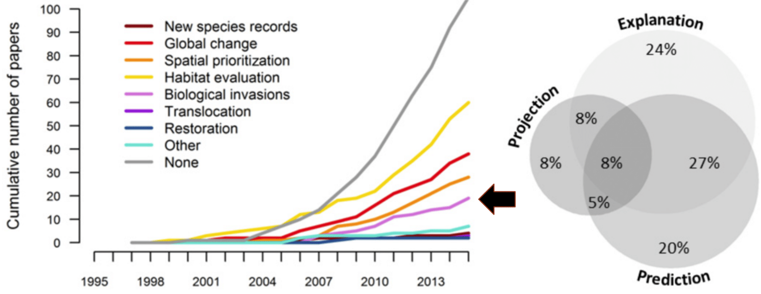
There is an entire group of methods that extend the idea of SDM by adding further information, or that are otherwise related to SDM. The main ones are:
1. Methods that model species interactions, accounting for biotic factors:
Further developments:
The Qb.SDM software package runs in the browser. There is no need to install any additional software to run a model - a browser (Chrome, Edge) is all you need.
2.1. Qb.SDM: quick start.Open the following link in your browser: https://wingeds.world/sdm
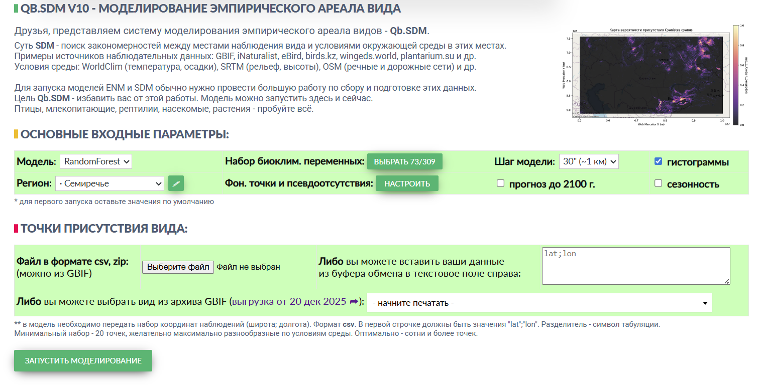
Qb.SDM is integrated with GBIF, the global biodiversity database. This means that for many species of animals and plants, Qb.SDM already has enough data to run a model and build a presence map for the species.
For a quick start, you can leave most settings untouched - you only need two steps:
1. In the “region” field, select the modelling area you are interested in. For a first try, it is recommended to pick a relatively small region, such as Semirechye or the Caucasus - this way you will see the result faster. 2. In the field at the very bottom, select a species. In the “start typing” box on the right, enter the name of the species you're interested in. Not every species in the database has a Russian-language name; if you cannot find a species, try its Latin name (the easiest way to find one is on the species' Wikipedia page).As an example, try leaving everything unchanged except for selecting the species “Azure tit (white-headed tit)” - and click “run model”:
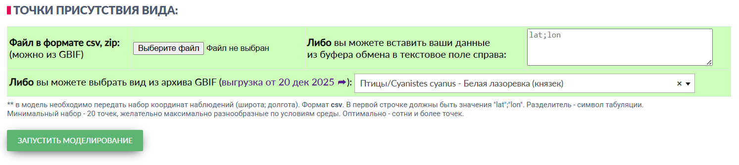
After a few minutes you will get a result that looks like this:
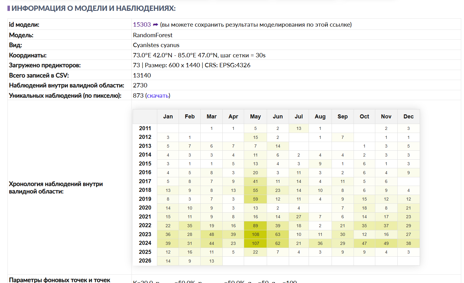
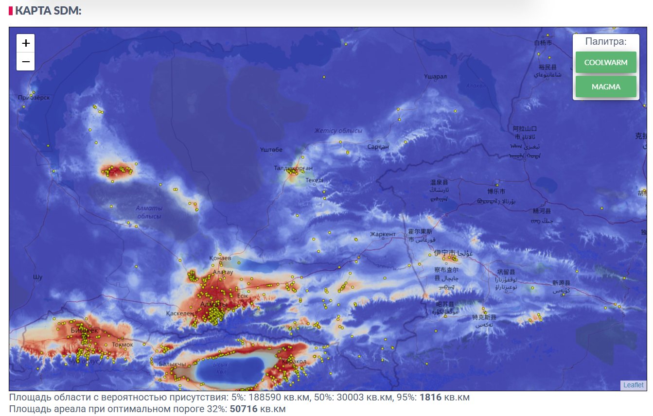
Example: SDM result for the azure tit (Cyanistes cyanus), modelling region - Semirechye [M2]
For more on presenting and interpreting results, see section 2.3.
The rest of this section covers how to set the input parameters more deliberately.
2.2. Qb.SDM: description of input parameters.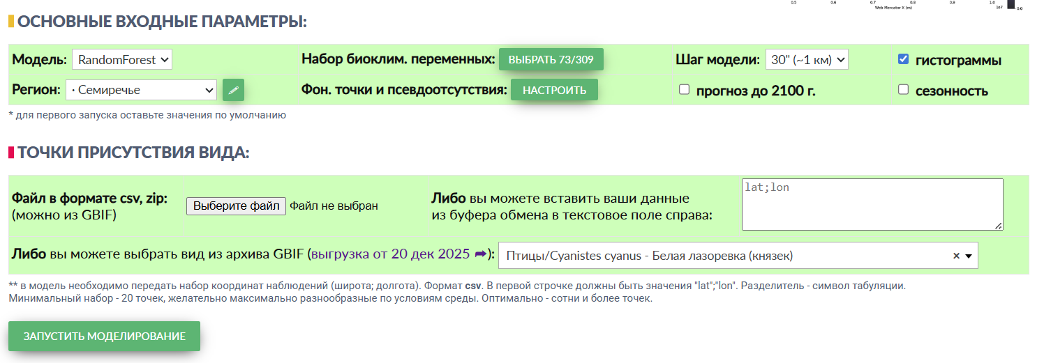
The model's main input parameters are shown above. If you are using GBIF data, it is enough to specify the region and the species - the system will then select the optimal parameters for modelling on its own.
For all other cases, let's look at the parameters in more detail.
2.2.1. “Model”. Three options are available here:
- RandomForest, an “ensemble of decision trees” - the default model. Produces the “softest” representation of the result and generally the best accuracy; - XGBoost, “gradient boosting” - the second default model. Often shows better accuracy than RandomForest, but draws the boundaries of a species' distribution more sharply, which may not correspond to real-world occurrences; - MaxEnt, “maximum entropy” - an alternative model. Where RandomForest and XGBoost tend to better describe a species' realized ecological niche (adjusted for observer effect), MaxEnt tends to better describe its fundamental niche (with the same adjustment). The CHELSA predictor set is not available for MaxEnt in Qb.SDM, and future-scenario modelling is not implemented for it either.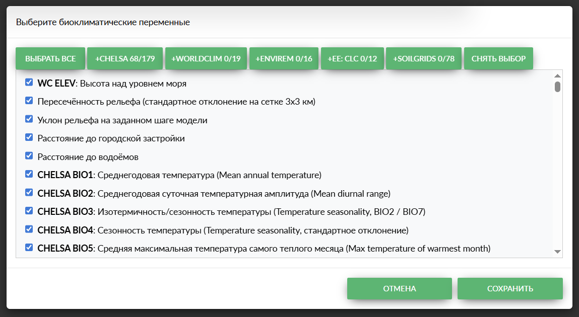
2.2.2. “Set of bioclimatic variables”.
The following variable sets are available:
- CHELSA [2] - the most up-to-date and complete set of bioclimatic variables, currently the recommended choice for SDM; - WorldClim [5] - one of the original base sets of bioclimatic variables, now almost universally superseded by CHELSA. Using CHELSA and WorldClim together serves no purpose; CHELSA is the preferred option; - ENVIREM [6] - a set of composite bioclimatic variables complementing WorldClim. It, too, is now being superseded almost everywhere by CHELSA; - EarthEnv LandCover [7] - a set of land-cover predictors: vegetation, water bodies, urban development, etc. Recommended for most species. An example where EE LandCover should be used with caution: when you need to clearly separate habitat suitability in cities from the human bias factor; - SoilGrids [8] - a set of predictors describing the physical and chemical composition of soils. Most important for terrestrial animals and plants.The MaxEnt model is sensitive to collinearity (co-dependence) between predictors, so its use of multiple predictors is limited, and it is recommended to add only one or two per run.
RandomForest and XGBoost are not sensitive to collinearity, so you can use practically all available predictors with them.
An important constraint: the number of unique observations should be noticeably larger than the number of predictors used. For example, if you only have 100 observations, it is recommended to limit yourself to 20-30 predictor layers.
2.2.3. “Model step”, options: 30” (arc-seconds, roughly 1x1 km), 1’ (arc-minute, roughly 2x2 km), 5’ (arc-minutes, roughly 10x10 km).
The coarser the step, the faster the model runs - and the coarser the result. For the best accuracy, a 30” step is optimal; however, when modelling large regions (for example, the whole of Kazakhstan or Russia), the model's resolution is limited to one arc-minute for performance reasons.
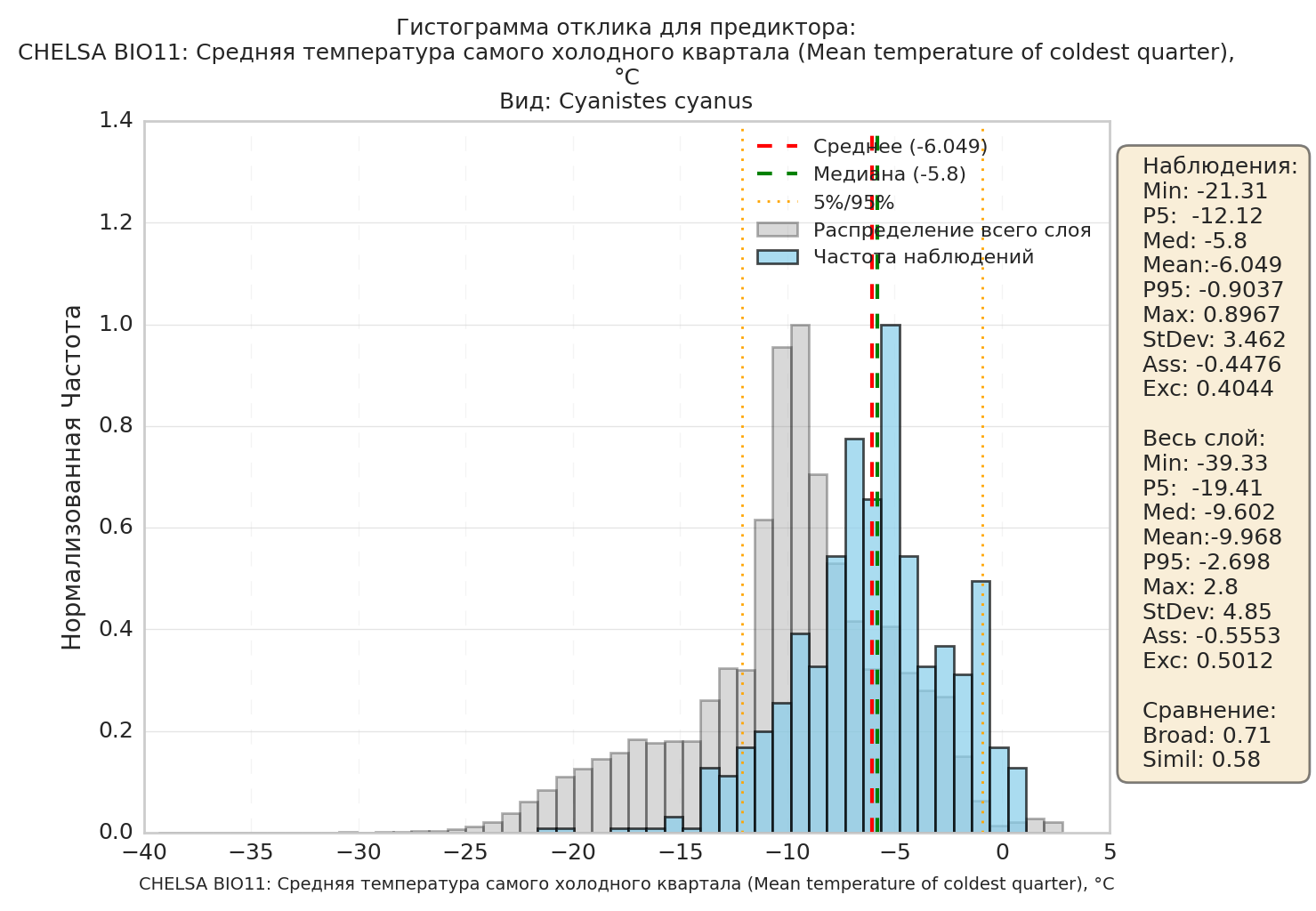
2.2.4. “Histograms”. If this option is checked, the system will build a histogram for every selected predictor layer. Histograms can provide extra information about a species' ecology, its preferred conditions, and the conditions available within the region.
The example shows that the azure tit prefers warmer conditions than are available on average across the modelling region. This means that this factor will be limiting its distribution.
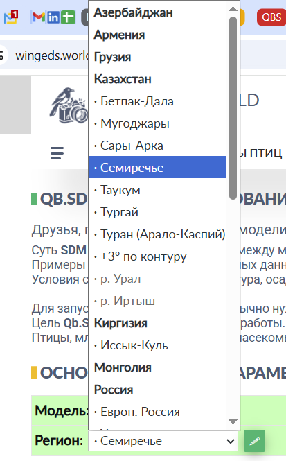
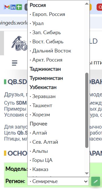
2.2.5. “Modelling region”. It is recommended to use one of the standard regions - there is a fairly wide selection to choose from.
If you did not find a suitable region in the list, you can specify your own by clicking the pencil icon to the right of the dropdown list:
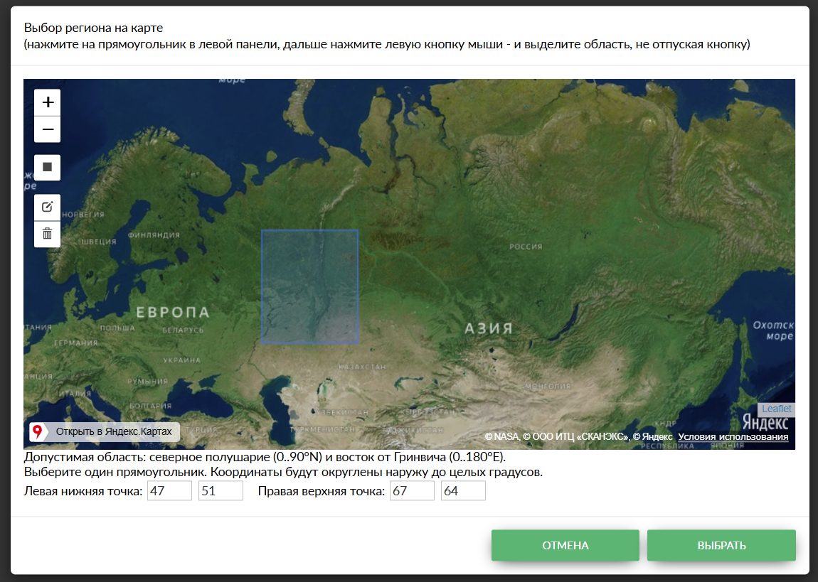
You can then click the grey square on the left and draw the region you need with the mouse, or enter the coordinates (latitude and longitude of the bottom-left and top-right points) manually.
For non-standard (manually drawn) regions, the size of the modelling area is limited by the bounding rectangle of the drawn shape: width along longitude, height along latitude. Three zones apply:
- up to 20×20 degrees - the area is allowed with any model step; - larger than 20×20, but no more than 60° of longitude and 30° of latitude - the area is allowed, but the model step is forced to 5’ (~10 km); - larger than 60×30 degrees - the area is not allowed; building the model is unavailable.Future-scenario modelling is also not performed for non-standard regions.
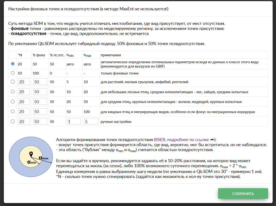
2.2.6. “Background and pseudo-absence points”. Running machine-learning algorithms requires two kinds of points. The first are points where the species is present - this is observation data, either yours or from GBIF. The second are points where the species is absent. The algorithm then learns to predict how likely the species is to occur at any given point.
Observation data usually contains only information on where the species is present, not where it is absent. However, there are several algorithms that can generate such points using statistical methods.
These algorithms take a number of parameters as input, which can be determined from knowledge of the species' biology. More detail is given in section 2.4.3.
Qb.SDM has a built-in algorithm that selects these parameters based on tabulated values for a group of species. For a first run you can rely on this algorithm (the first item in the “auto” list), or choose one of the preset parameter sets. Fully manual control of these parameters is also possible. Section 2.4.3 describes some heuristics on this subject.
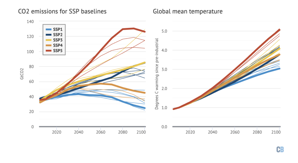
2.2.7. “Forecast to 2100”. Climatologists have developed a set of scenarios for how Earth's climate may change through 2100, the so-called SSPs - “Shared Socioeconomic Pathways” [9]. They model humanity's “behaviour” on a global scale, and, as a result, how key climate variables - mean temperature, precipitation, etc. - will change.
In the context of SDM, SSP scenarios are of interest because the providers of the main bioclimatic variable sets (CHELSA, WorldClim and others) have prepared predictor sets modelling different future scenarios [10].
Qb.SDM includes a future model from CHELSA for three scenarios: SSP1-2.6 (optimistic), SSP3-7.0, and SSP5-8.5 (pessimistic). Checking this option gives you forecasts of changes in species presence for these three scenarios, for three periods: 2011-2040, 2041-2070, 2071-2100.
Which scenario will turn out to be closest to reality cannot be reliably predicted in advance - it depends on future climate policy and socio-economic factors. In the absence of additional information specific to a given region or species, it is recommended to treat all three scenarios as equally likely and to compare results between them, rather than relying on any one of them.
It is also worth keeping in mind: the SSP3 scenario carries not just an emissions level (7.0 W/m²), but also a socio-political storyline - “Regional Rivalry” - world fragmentation, rising nationalism, and weakening international cooperation. A number of observers have noted that this particular scenario came to look more plausible during the 2020s, amid rising geopolitical tension and deglobalization - regardless of whether the actual pace of emissions growth matches the figure projected for SSP3-7.0.
2.2.8. “Seasonality”. Checking this option gives you, in addition to the base model, a set of 12 models - one per month. Such models can be of interest, for example, when studying migratory or nomadic species.
Modelling seasonality is only worthwhile if you have at least a few hundred observations.
2.2.9. “Species presence points”. The system allows three ways to enter observation data:
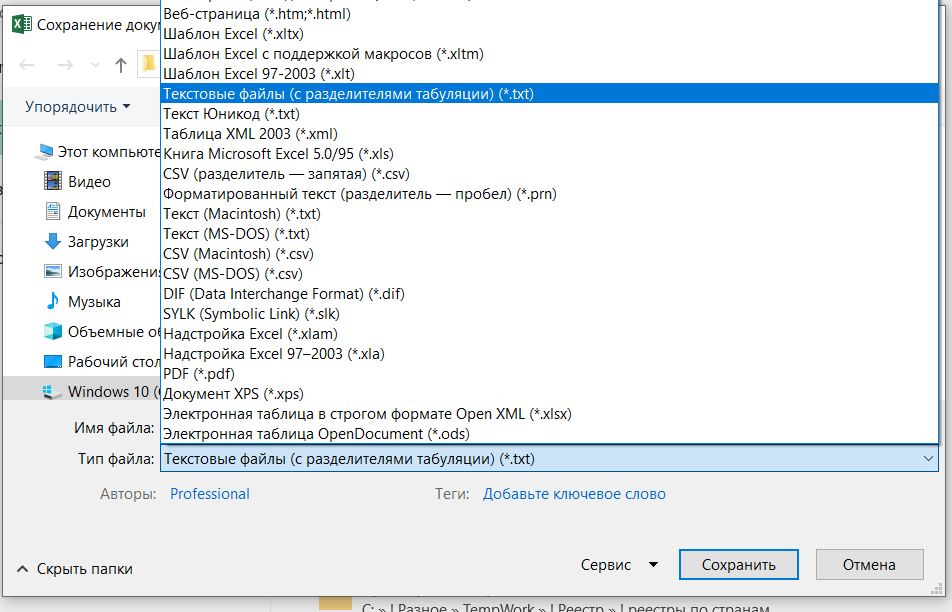
2.2.9.1. Upload a file in CSV format. The file must contain at least two fields: “lat” and “lon” - the latitude and longitude of the observations as decimal coordinates. The decimal separator is a dot. The cell separator is a tab character.
Important: if you are saving data from Excel, you need to select this option:
Example of a correctly formatted file:
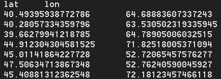
2.2.9.2. Second option: paste data in the same format into the “paste data from clipboard” field.
The result will look something like this:

2.2.9.3. Third option: select existing data from the GBIF archive. Enter the name of the species you're interested in into the “start typing” field. Not every species in the database has a Russian-language name; if you cannot find a species, try its Latin name (the easiest way to find one is on the species' Wikipedia page).
The result will look something like this:

2.2.10. “M-factor (habitat accessibility)”.
In addition to abiotic habitat suitability (climate, soil, terrain - what the machine-learning model evaluates directly), Qb.SDM can additionally take into account how physically reachable that habitat is for the species, based on its known observation points. This is a separate multiplier from 0 to 1, by which the final suitability map is multiplied: final map = abiotic suitability × M-factor.
The M-factor approximately computes the “cost of travel” from the nearest observation point to every point on the map, taking into account:
- the species' dispersal distance (km) - set separately for the current period and for each of the three future forecast periods (2011-2040, 2041-2070, 2071-2100), generally increasing over time;
- terrain - steep slopes increase the “cost” of movement;
- elevation barriers - the species cannot cross a mountain pass or depression whose elevation differs substantially from that of the points where it was observed (with some allowance for climate warming);
- water barriers - for most species, open water is a barrier; this barrier is ignored for birds, while for semi-aquatic classes (such as amphibians) water becomes, instead, a dispersal “corridor”;
- observer bias (optional) - an additional penalty can be applied to areas with low observer activity, so as not to confuse “the species isn't there” with “nobody looked there”.
Default values are selected automatically based on the species' class/kingdom (similarly to the background-point parameters, see sections 2.2.6 and 2.4.3), but can also be set manually. The M-factor can be adjusted, or disabled entirely - in which case the map shows only abiotic habitat suitability, with no accessibility correction. For a technical description of the algorithm, see section 2.4.4.
2.3. Qb.SDM: presenting and interpreting results. 2.3.1. The “modelling results” section.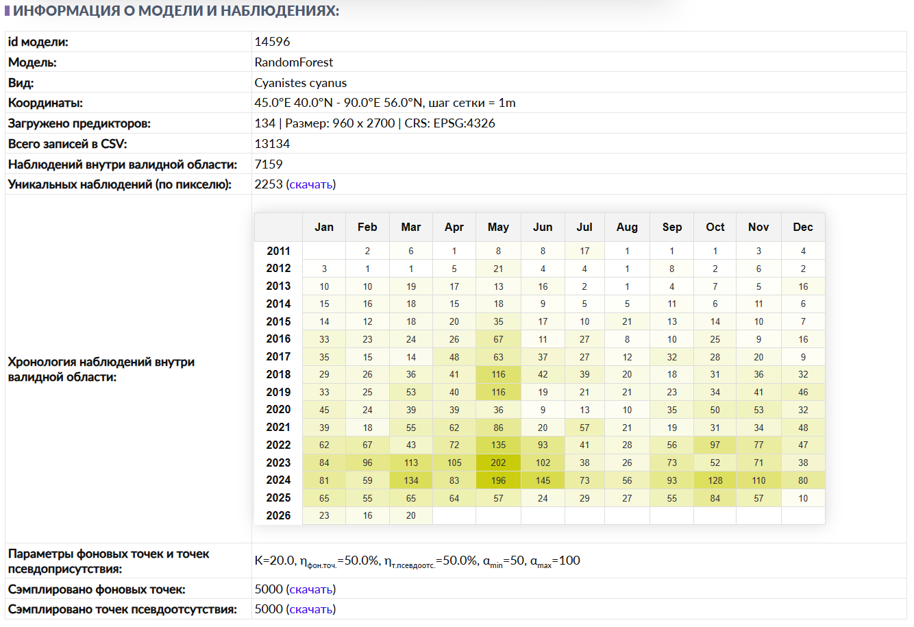
The “modelling results” section presents information about the input data submitted, a brief summary of the observations, and the metrics - scores assessing the model's quality.
2.3.1.1. The “model id” line gives a link to the current model. You can copy and save this link to return to this run later. Example link: https:/wingeds.world/sdm/14047
2.3.1.2. The “model” line shows which model performed the computation. Options:
- RandomForest; - XGBoost; - MaxEnt.2.3.1.3. “Species” - the biological species the model was run for. This field has no direct effect on the computations. The species information is taken from the species field of the uploaded CSV file (or from GBIF data, if the source data was selected from the GBIF archive).
2.3.1.4. “Coordinates” - the geographic coordinates and grid step size of the modelling area.
2.3.1.5. “Predictors loaded”. The first number (24) is how many predictors were selected for this modelling session. It is followed by the size of the predictors in raster points (600x1440) and the geographic projection of the rasters.
2.3.1.6. “Total records in CSV” - the total number of observations in the archive. Note that not all observations necessarily fall within the specified modelling area.
2.3.1.7. “Presences within the valid area” - the total number of observations from the archive that fall within the specified modelling area.
2.3.1.8. “Unique presences per pixel”. The logic of SDM is to take the values of the biogeographic variables at the species' presence points and use this information to determine suitable habitat.
However, predictor layers come at a limited spatial resolution (for example, a cell of 30x30 arc-seconds), so there is no point computing the value of a given predictor cell more than once.
Therefore, the total number of observations within the valid area is split by predictor cell, keeping only one observation per cell.
2.3.1.9. “Observation history” - the number of observations by month within the specified modelling area.
2.3.1.10. For more on background points and pseudo-absence points, see section 2.4.3.
This block provides the following information:

K=20 - how many times more background and pseudo-absence points to generate, relative to the number of unique observations.
nbackgr.pts=50% and npseudo-abs.=50% - the share of background points and pseudo-absence points, respectively. They sum to 100%.
For example, if there were 25 unique observations, K=20, n=50%, then 25 x 20 = 500 background + pseudo-absence points will be generated (250 background and 250 pseudo-absence).
αmin=50 and αmax=100 - the distance, in raster-cell units, within which pseudo-absence points will be generated.
The total number of background and pseudo-absence points does not exceed 10,000; this limit is set programmatically.
2.3.2. The “quality metrics” section.2.3.1.11. The next block shows the model's quality metrics:
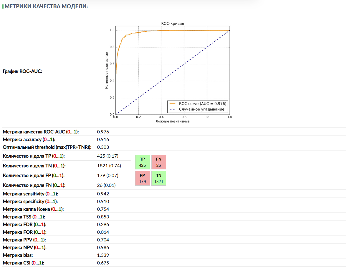
The ROC-AUC chart and metric shows the relationship between the true positive rate (TPR, or sensitivity) and the false positive rate (FPR) as the classification threshold changes. AUC (Area Under the Curve) is the area under this curve.
Interpretation:
- ROC-AUC = 1: A perfect model, separating the classes without error. - ROC-AUC > 0.9: An excellent model. - 0.8 < ROC-AUC <= 0.9: A very good model. - 0.7 < ROC-AUC <= 0.8: A good model. - 0.6 < ROC-AUC <= 0.7: An acceptable model. - 0.5 < ROC-AUC <= 0.6: A weak model, barely better than random guessing. - ROC-AUC = 0.5: The model performs like random guessing (for binary classification). - ROC-AUC < 0.5: The model performs worse than random guessing (the classes may have been swapped, or there is a serious problem).For species distribution modelling tasks, especially under complex natural conditions, ROC-AUC values above 0.9 are considered good. Values above 0.95 are excellent. Anything below 0.7 requires careful analysis and, most likely, a change in model settings and the addition of more observation data.
The accuracy metric = (TP + TN) / Total. The overall share of correct predictions.
Optimal threshold. The output of an SDM model is a map with presence-probability values from 0 to 1. But which value should be chosen as the cutoff above which we can declare the habitat suitable for the species? This is a computed value that maximizes the share of correct predictions. For all points where the presence probability is above the optimal threshold, the species can be assumed to be present.
The count and share of True positives (TP, TPR) - the number and share of points where the species is present and the model predicted it correctly.
TN (TNR) - the number of points where the species is absent, and the model predicted absence.
FP (FPR) - the number of points where the species is absent, but the model incorrectly predicted presence.
FN (FNR) - the number of points where the species is present, but the model incorrectly predicted absence.
NB: In Qb.SDM, as in most SDMs trained only on presence data, the role of “absence” is played by background points and pseudo-absence points (see sections 2.2.6, 2.4.3) rather than confirmed field data on absence. Because of this, TN and FP in the formulas above are conditional quantities: “the model predicted presence/absence at a point that is treated as an absence solely by construction of the sample.” All metrics that use TN or FP (specificity, accuracy, Cohen's Kappa, TSS, FOR, NPV, bias, CSI) are therefore an approximation, not a strict evaluation against verified field absence data. The threshold scales for interpretation given below (adapted from the classic Swets, 1988 grading) were originally derived for tasks with true absences; for presence-background models, the maximum achievable AUC/Kappa/TSS value depends on the background-to-presence ratio and on the size of the modelling region, so the “good/excellent” boundary should be treated as a rough guide rather than a strict standard (for more on this criticism, see [13], [14]).
Metric sensitivity = TP / (TP + FN) - sensitivity.
Metric specificity = TN / (TN + FP) - specificity.
Cohen's Kappa measures the degree of agreement between the actual and predicted presences, corrected for the agreement expected by chance. This is especially useful when classes are imbalanced (few observation points).
- Kappa = 1: Perfect agreement. - 0.8 < Kappa <= 1: Almost perfect agreement. - 0.6 < Kappa <= 0.8: Substantial agreement. - 0.4 < Kappa <= 0.6: Moderate agreement. - 0.2 < Kappa <= 0.4: Fair agreement, though above chance. - 0 < Kappa <= 0.2: Agreement close to chance. - Kappa = 0: Agreement identical to chance. - Kappa < 0: Agreement worse than chance (rare, but possible with a poor model).For species distribution modelling, Kappa values above 0.6 are considered good, and above 0.7 very good. Scores above 0.8 are excellent.
Cohen's Kappa accounts for chance agreement, which makes it a stricter metric than plain accuracy (or ROC-AUC), especially under strong class imbalance. For example, if 95% of the territory is unsuitable for the species, a model that predicts “absence” everywhere will have high accuracy (95%), but a low Kappa.
TSS (true skill statistic) is a metric that sums sensitivity (TPR) and specificity (True Negative Rate, TNR). TSS = TPR + TNR - 1.
- TSS = 1: A perfect model (100% sensitivity and 100% specificity). - TSS > 0.8: An excellent model. - 0.6 < TSS <= 0.8: A very good model. - 0.4 < TSS <= 0.6: A good model. - 0.2 < TSS <= 0.4: An acceptable model. - 0 < TSS <= 0.2: A weak model. - TSS = 0: The model performs like random guessing (i.e. sensitivity + specificity = 1). - TSS < 0: The model performs worse than random guessing.For species distribution modelling, TSS values above 0.6 are considered good, and above 0.7 very good. Scores above 0.8 are excellent. TSS is very sensitive to how well the model predicts both positive and negative cases, which makes it valuable for assessing prediction accuracy on both sides of the distribution.
The FDR metric (False Discovery Rate) = FP / (TP + FP). Reflects the share of false positives among everything the model predicted as positive. Important when a false detection is very costly.
The FOR metric (False Omission Rate) = FN / (TN + FN). Reflects the share of false negatives among everything the model predicted as negative. Important when missing a true case is very costly.
The PPV (Positive Predictive Value) metric = TP / (TP + FP). The percentage of true positives among everything the model predicted as positive. The inverse of FDR.
The NPV (Negative Predictive Value) metric = TN / (TN + FN). The percentage of true negatives among everything the model predicted as negative. The inverse of FOR.
The bias metric = (TP + FP) / (TP + FN). The ratio of predicted events to actual events:
- BS = 1 means an unbiased forecast (the number of predicted positives matches the number of actual positives); - BS > 1 means the model predicts more positives than there actually are (bias toward positives); - BS < 1 means the model predicts fewer positives than there actually are (bias toward negatives).The CSI (Critical Success Index) metric = TP / (TP + FN + FP). Reflects the share of correctly predicted events among all events (true and false). Well suited for assessing the forecasting of rare events.
2.3.3. The “response curves” section.Each predictor layer in SDM characterizes one of the biogeographic variables. For example, the CHELSA BIO1 layer is mean annual temperature in degrees. Its value is given for every point on Earth's surface, or more precisely for a cell measuring 30x30 arc-seconds (slightly less than 1x1 km):
As an example, take the Semirechye region - it covers Lake Balkhash and Lake Alakol, as well as the rivers flowing into these lakes from the Trans-Ili Alatau mountain system. The dominant colour on the map is red. According to the scale, the region's mean annual temperature ranges from 5 to 12 degrees. However, there are a few white, and even blue, areas where the mean annual temperature is below -10 degrees. These are the glaciers of the Tian Shan, located above 4,000 metres.
The boundaries of Semirechye in geographic coordinates: 73.0°E 42.0°N - 85.0°E 47.0°N. The sector measures 12 degrees of longitude by 5 degrees of latitude, or 300 x 620 arc-minutes, or 600 x 1440 points of the CHELSA BIO1 predictor. In other words, from the SDM model's point of view, the size of the BIO1 layer is 600 x 1440 = 864,000 points.
We can divide the temperature scale into, say, 1-degree bins: 0-1, 1-2, 2-3, 3-4 degrees, and so on. For each bin we count the number of points whose temperature falls within it, for example 0-1 degree: 2,000 points, 1-2 degrees: 2,100 points, 2-3 degrees: 2,500 points, and so on. The exact number of points is not especially interesting on its own (it depends on scale); what matters is the distribution relative to the bin with the largest count.
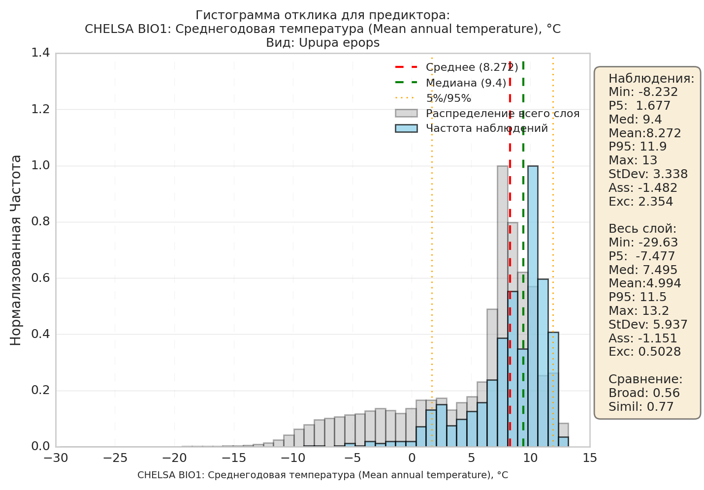
Performing this operation for all bins gives us the response histogram for the predictor. In the image above, this is the grey-filled histogram - it shows how the predictor's values are distributed across the background, i.e. across the entire modelling area.
Next, we take only the points where the species was observed, and perform the same operation on them. For the 0-1 degree bin: 80 observations, 1-2 degrees: 120 observations, 2-3 degrees: 160 observations, and so on. As with the background points, the exact counts are not especially interesting on their own; we build the distribution relative to the bin with the largest number of observations.
In the image above, this is the blue-filled histogram - it shows how the species' observations are distributed across this climate layer.
You can see that the peak of the “blue” distribution sits around 10 degrees, to the right of the peak of the “grey” distribution (7 degrees). The same holds for the mean values, given in the table on the right (mean): 8.272 degrees for observations versus 4.994 for the entire layer.
It is also apparent that the species has almost no observations below 0 degrees, whereas the background histogram extends well below 0 degrees - down to roughly -15.
Comparing the background histogram with the observation histogram tells us about the species' ecology, with respect to this layer, within this region. In this case, we can see that our species “avoids” low-temperature areas, i.e. the mountains, preferring warmer, lowland areas.
The ecological meaning of the most commonly encountered situations:
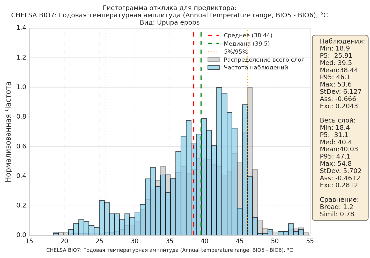
2.3.3.1. The “blue” and “grey” histograms look similar across the entire range of presence (in the table, Broad and Simil are close to 1). This means that, for this predictor, conditions across the region (“in E-space”) are, on the whole, comfortable for the species.
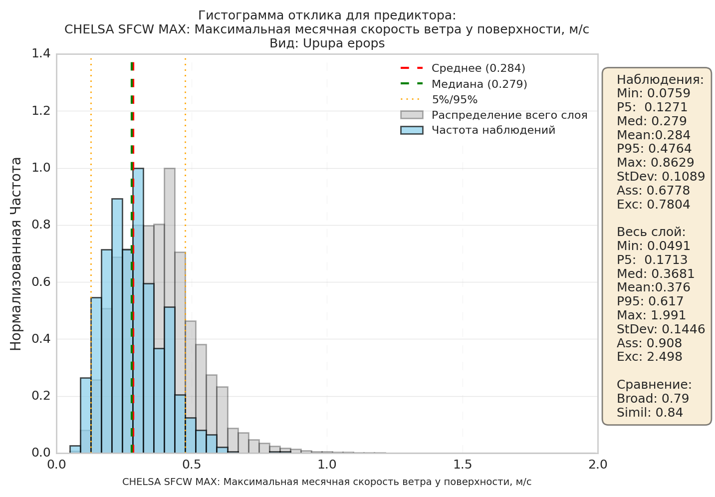
2.3.3.2. Both histograms resemble each other, but appear shifted (the peaks do not coincide). In the table, Simil is close to 1, but Med/Mean differ between observations and the full layer. This means that, for this layer (“in E-space”), the species is more comfortable within some limited range. On the map, this will show up as one or several isolated areas (“in G-space”).
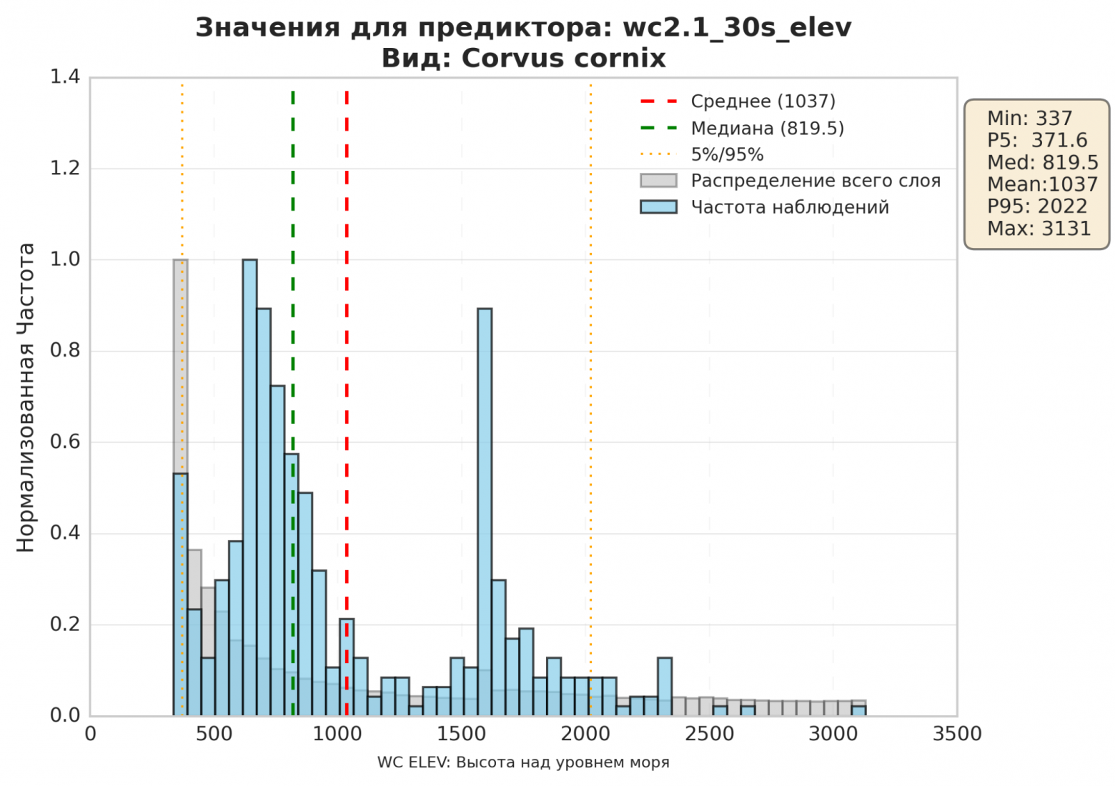
2.3.3.3. The background layer (grey) is distributed as a single-peaked “bell curve”, while the observations (blue) show two distinct peaks, located far apart from one another.
In effect, this histogram shows two different ecological niches overlaid on top of each other. A graph like this requires further investigation before it can be interpreted. The most common situations are:
- we are seeing the species' seasonal migration or nomadic movement within the modelling area - the species lives in one area in summer and another in winter; - the graph shows two different populations adapted to different conditions. For example, selection may have caused two different species to end up in the model. Or two different subspecies (populations) of the same species, living under different conditions - possibly in the process of forming reproductive isolation.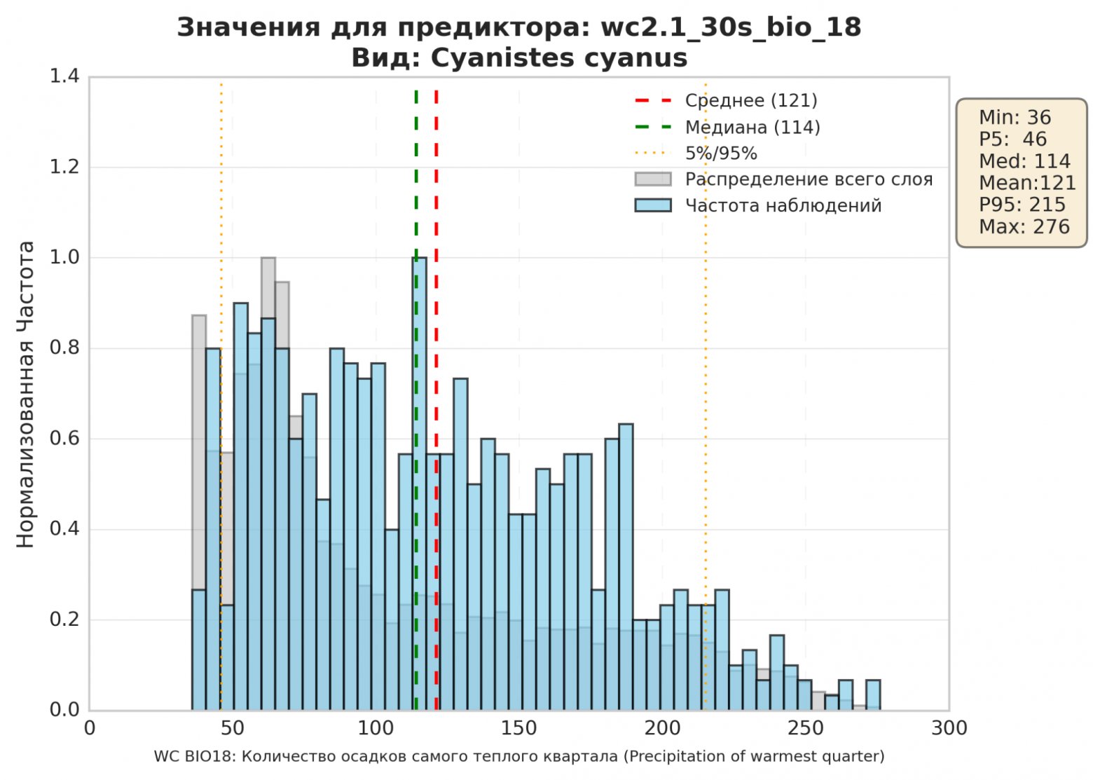
2.3.3.4. The histogram is evenly “smeared” across all values. The ecological meaning of such a graph is that the species is practically independent of this factor. It is comfortable at almost any level of precipitation, as long as it does not exceed roughly 200 mm per quarter.
Description of the values in the table to the right of the histogram:
- “observations” - the top half of the table statistically describes the species' occurrences (the blue histogram); “full layer” describes the modelled region as a whole (the grey histogram); - min and max - the minimum and maximum predictor value (in this example, the minimum temperature where the species was observed is Min=-8.232 degrees, while for the full layer Min=-29.63 degrees; the maximum temperatures for observations and the full layer, by contrast, nearly coincide); - P5, P95 - the values below which >5% and <95% of all points fall (in this example, P5 for observations is 1.677 degrees, while for the full layer P5=-7.477 degrees, i.e. the species does not care for cold regions); - Med - median, Mean - mean value; - StDev - standard deviation. A larger standard deviation indicates a wider spread of values around the mean within the given set; correspondingly, a smaller value indicates that values are clustered closely around the mean; - Ass - skewness coefficient. Positive if the right tail of the distribution is longer than the left, negative otherwise. Zero for symmetric distributions; - Exc - kurtosis coefficient. A measure of how sharp the peak of the distribution is; - the “comparison” block provides statistical measures comparing the two histograms (blue and grey) with each other; - Broad - the relative width of the histograms; the closer to 1, the closer the two histograms' widths are to each other; - Simil - the similarity (correlation) coefficient of the histograms, where 1 means direct proportionality. 2.3.4. The “predictor importance” section.Not all predictors (bioclimatic variables) are equally important for predicting a species' presence.
For example, for semi-aquatic species, proximity to water bodies will be one of the most important predictors. If you run the model without the “distance to water bodies” predictor, the model's quality (accuracy) will most likely drop sharply.
Conversely, for desert species, predictors describing the degree of deciduous or coniferous tree cover will be practically unimportant. Running the model without them will barely change its quality.
The SDM model can compute an importance score for each predictor. The computation works as follows: the model looks at how strongly a change in that predictor affects the change in the final result.
Predictor importance is another measure that lets you draw conclusions about a species' ecology:
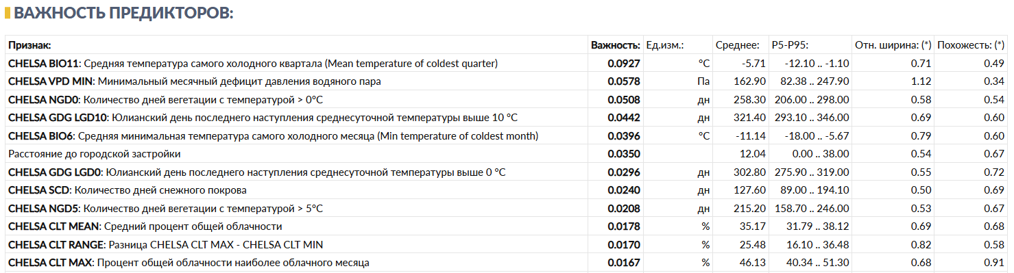
In this example, the most important predictor for the modelled species (the Eurasian hoopoe, Upupa epops) turns out to be BIO11, the mean temperature of the coldest quarter. This species cannot survive in regions with too low a winter temperature.
Note that the second- and third-most-important predictors here do not affect this species directly. They influence the species' distribution indirectly, for example through trophic chains (the hoopoe is an insectivorous bird).
NB: It is important to understand the limitations of this metric. RandomForest, XGBoost and MaxEnt define importance mathematically in different ways (for decision trees, it is a predictor's contribution to reducing uncertainty at splits; for MaxEnt, it is the feature's weight after regularization), so importance percentages for the same predictor cannot be directly compared across different models. Second, if two predictors are strongly correlated with each other (for example, mean annual temperature and the mean temperature of the warmest month), the model may “split” the importance between them in an arbitrary way - a low importance score for a particular layer does not necessarily mean that the corresponding ecological factor is unimportant to the species; it may instead mean that a correlated predictor has taken over its role within the model.
The remaining numbers in the predictor importance table match the numbers from the response histograms, see section 2.3.3.
2.3.5. The maps section.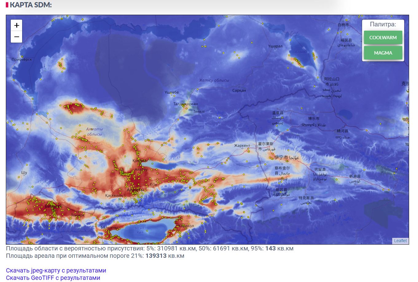
The map is the result of projecting E-space (suitable ecological niches) into G-space (geographic space).
In much of the SDM literature, the model's output is called the probability of species presence; however, from an ecological point of view this is not accurate. What the map actually represents is suitable habitat (according to the model and the set of predictors fed into it).
Areas shown in blue are areas where conditions are unsuitable for the species (0% suitability). Red marks the best match (100% suitability).
Yellow dots mark the species' observations that were fed into the model.
Note that a number of yellow markers fall within blue areas. These may be either (systematic) model errors or erroneous observations. In some cases a species may be observed outside its suitable habitat, for example during migration or while fleeing a predator.
The reverse situation is also possible, where red areas have no markers at all. Possible reasons, besides model inaccuracy: there were no observers in that area able to recognize this species. Or the species cannot reach that area due to some constraint (for example, crossing a sea or a mountain range).
For more detail, see section 1.2.
Also pay attention to the “range area at the optimal threshold” result. The threshold value is the probability cutoff at which the model shows its highest predictive power. In other words, it is most likely that taking all points above this threshold will give you the species' actual range area.
Future maps. If the “Forecast to 2100” option was checked when the run was started (see 2.2.7), the “Future” section shows three scenarios - SSP1-2.6, SSP3-7.0 and SSP5-8.5 - each for three periods: 2011-2040, 2041-2070, and 2071-2100. For each scenario, separate maps are available per period, together with an animation (GIF/MP4) assembled from these maps. A single area table for suitable habitat shows the value for each period and scenario, along with the percentage change relative to the current map (the “Now” period). As with the current map, the value is given both for the optimal threshold (see 2.3.2) and for a soft threshold (half the optimal value, a less strict habitat-suitability criterion) - in practice, for most models the areas at both thresholds are the same or close. An increase in area does not necessarily mean the species' situation is improving: some of the newly suitable habitat may be physically unreachable for the species - for more detail, see 2.4.4, covering the M-factor. The “area over time” chart below the table shows all three scenarios on a single year axis - for compactness, the points on the chart correspond to the same three periods, labelled for simplicity as 2040/2070/2100.
Past maps. The “Past” section is available if the corresponding option was checked when the run was started, and shows how the area of suitable habitat has changed over the last 20,000 years, based on the CHELSA-TraCE21k [4] climate dataset - a separate dataset unrelated to the model's other predictors. Because of this, the area shown on the “Now (per TraCE21k)” card typically does not match the area on the model's main (current) map - this is expected, and not an error, since the two climate datasets are independent of one another. The gallery shows five characteristic periods (20,000, 10,000, 2,000 and 1,000 years ago, and the present), and the chart below the gallery shows the full history across every time point the data source provides.
Seasonal maps. The “Seasonality” section is available if the “Seasonality” option was checked when the run was started (see 2.2.8), and shows 12 separate models - one per month, each built from that month's observations and climate data. This view is useful for migratory and nomadic species, since it reveals the seasonal shift in suitable habitat. Months for which too few observations were collected are flagged as less reliable, and their maps should be trusted with caution.
2.4. Qb.SDM: technical description of the algorithms:The current source code of Qb.SDM is available on Github at https://github.com/mad-kiba/python-sdm/. If you would like to reproduce the algorithm or install Qb.SDM on your own machine, the Github documentation provides detailed instructions for doing so. You can also use Qb.SDM as a plug-in module in your own projects, provided you credit the Github repository.
A general description of the Qb.SDM algorithm is given in section 2.4.5.
2.4.1. Observation pre-processing. 1. If the file has a species column and all its values are the same, the model takes the species name from it. 2. If the file has kingdom and class columns and the values within each are the same, the model takes the kingdom and class names from them, which are used to compute the species' pseudo-absence points, see 2.4.3. 3. For coordinates, the columns named lat and lon are used. If the file has no such columns, the pairs Latitude/Longitude, latitude/longitude, decimalLatitude/decimalLongitude are used instead. 4. Observations for which the coordinateUncertaintyInMeters field is set, and its value is greater than 1000 metres, are removed from the sample (since the model's minimum step is 30 arc-seconds, roughly 1x1 km). 5. Observations with collectionCode = EOA are removed from the sample (GBIF data published under this collection has incorrect coordinates). 6. Observations with no year specified, as well as those made before the year 2000, are removed from the sample. 7. If fewer than 10 points remain in the sample, the model stops. 8. All observations falling within the same raster cell are removed except one - deduplication. 9. If fewer than 5 unique points remain after deduplication, the model also stops. This check is separate from check 7: several original observations can land in the same raster pixel (especially with a coarse model step, such as 5'), and after deduplication the number of unique points may be noticeably smaller than the number of records in the original file. 2.4.2. Predictor pre-processing.The target CRS is EPSG:4326 - a geographic coordinate system based on the WGS 84 ellipsoid, in which point positions are given as latitude and longitude in decimal degrees.
If a predictor's projection differs from EPSG:4326, it is reprojected.
Running a machine-learning algorithm requires two kinds of points:
- points where the species is present; - points where the species is absent.Based on these points, the algorithm learns to predict how well the conditions at any point on the map match the first or second class, i.e. how likely the species is to be found there.
Presence points are fairly straightforward - this is observation data, whether yours, from GBIF, or from any other source. The main requirement for observation data is, in essence, that its spatial resolution be higher than that of the predictor layers. With GPS built into most modern smartphones, this requirement is met with plenty of margin.
Absence points are a considerably harder matter. Technically, GBIF can hold absence records for a species, but in practice such records make up only about 0.01% of entries - and they do not even exist for every class of animal or plant.
Except in trivial cases (“fish live in water”), it is quite difficult to guarantee that a species does not occur at a given point (i.e. within a 1x1 km cell) - especially if it occurs at neighbouring points.
The problem is so serious that, for a long time, the leading SDM algorithm was MaxEnt - with fairly mediocre quality, but one that, in theory, does not require absence points. However, MaxEnt has other drawbacks, such as its intolerance of collinearity between predictors.
As a result, several algorithms emerged that can generate “absence” points for a species using statistical methods. Two of them are the main ones:
- the background-point method; - the pseudo-absence-point method.2.4.3.1. The background-point method. This method is fairly straightforward: “absence” points for the species are drawn from across the entire region at random (in the background), excluding the presence points.
It might seem that this method should not be very accurate; however, in most cases it delivers better accuracy than MaxEnt given comparable input data. And the finer the model's resolution, the larger the share of points where the species is genuinely absent.
2.4.3.2. The pseudo-absence-point method (RSEB):

Around every presence point, a zone is formed where the species could plausibly occur but was not observed. This zone (a “ring” between αmin and αmax) is treated as the pseudo-absence zone.
It is recommended to set the αmin, αmax-αmin range to 10-20% of the distance the species can travel over its lifetime (or per season), or 100% of its possible daily movement range. Typically αmax = 2 * αmin. For more detail, see [11], [12].
The pseudo-absence-point method significantly improves model quality, but using it requires knowledge of the species' biology.
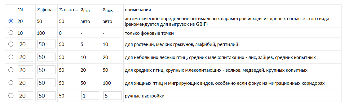
Qb.SDM includes averaged αmin and αmax values for different classes of animals and plants. However, if you are able to refine these values for your target species, it is recommended that you do so.
By default, the system attempts to automatically determine the animal's class and a suitable Amin and Amax value for it. An equal number of background points and pseudo-absence points is then generated. The number of each is set to 10 times the number of unique presence points, but no more than 10,000 in total.
For a first run you can rely on this algorithm (the first item in the “auto” list), or choose one of the preset parameter sets. Fully manual control of these parameters is also possible.
2.4.4. Accounting for species mobility (the M-factor).In addition to the statistical habitat-suitability model (the abiotic component, “A” in the BAM framework - Biotic-Abiotic-Movement, Soberón & Peterson), Qb.SDM implements a simplified treatment of the movement component (“M” - Movement): the species' physical ability to reach a suitable area.
The computation builds a “cost-distance” field from the species' presence points across the entire map: the speed of movement at each point depends on the terrain's slope and on the presence of elevation barriers and water barriers. The resulting field is converted into a multiplier ranging from 0 (unreachable) to 1 (matches an observation point), by which the suitability map is multiplied:
final suitability map = (abiotic suitability, from the statistical model) × (M-factor, from the accessibility field).
NB: This is not a fully mechanistic dispersal model, but a heuristic approximation: the default parameters (dispersal distance, elevation barrier, slope-penalty steepness) are set as averages by species class/kingdom, and may not reflect the specifics of a particular species or region. If data on the species' biology is available, it is recommended to set these parameters manually (see section 2.2.10).
2.4.5. Description of how the model works.The overall sequence of steps:
1. Prepare the predictor layers, bringing them to a common resolution and format, and standardizing the layers. 2. Load the observations. 3. Perform initial filtering of the observations. 4. Load the predictors. 5. Project the observations onto the predictors, computing the biogeographic variables at the observation points. 6. Deduplicate observations by predictor raster cell. 7. Generate background points and pseudo-absence points. 8. Build the response histograms. 9. Train the model. 10. Compute the model's quality metrics. 11. Apply the model to every raster point for the static predictors + present-time predictors. Build the species presence map. 12. >> for the static predictors + future-time predictors. Maps. 13. >> for the static predictors + monthly predictors. Maps. 14. Save the results and present them to the user.A detailed online course on SDM/ENM by the authors of the method:
https://www.youtube.com/playlist?list=PLCq9UxocboXPdulJteLT7MYj1WrW_tKcd
Course description and syllabus: Peterson A. et al. ENM2020: A FREE ONLINE COURSE AND SET OF RESOURCES ON MODELING SPECIES NICHES AND DISTRIBUTIONS. https://doi.org/10.17161/bi.v17i.15016
Other sources used:
1. A. Townsend Peterson & Jorge Soberón. Species Distribution Modeling and Ecological Niche Modeling: Getting the Concepts Right. https://doi.org/10.4322/natcon.2012.019
2. Brun, P., Zimmermann, N. E., Hari, C., Pellissier, L., Karger, D. N. (2022). CHELSA-BIOCLIM+ A novel set of global climate-related predictors at kilometre-resolution. EnviDat. https://www.doi.org/10.16904/envidat.332 https://www.chelsa-climate.org/
3. Khondamir Rustamov. Comparison of different models in predicting habitat suitability of rare species in Uzbekistan: 8 rare Tulipa species case-study. https://doi.org/10.1101/2022.07.08.499262
4. Karger, D. N., Nobis, M. P., Normand, S., Graham, C. H., and Zimmermann, N. E.: CHELSA-TraCE21k – high-resolution (1 km) downscaled transient temperature and precipitation data since the Last Glacial Maximum, Clim. Past, 19, 439–456, https://www.chelsa-climate.org/datasets/chelsa-trace21k-centennial-bioclim
5. WorldClim 2.1. Fick, S.E. and R.J. Hijmans, 2017. WorldClim 2: new 1km spatial resolution climate surfaces for global land areas. International Journal of Climatology 37 (12). https://www.worldclim.org/data/worldclim21.html
6. ENVIREM. Title P.O., Bemmels J.B. 2018. ENVIREM: an expanded set of bioclimatic and topographic variables increases flexibility and improves performance of ecological niche modeling. Ecography. 41:291–307. https://envirem.github.io/
7. EarthEnv Land Cover. Tuanmu, M.-N. and W. Jetz. 2014. A global 1-km consensus land-cover product for biodiversity and ecosystem modeling. Global Ecology and Biogeography 23(9): 1031-1045. https://www.earthenv.org/landcover
8. SoilGrids. Common soil chemical and physical properties: Poggio, L., de Sousa, L. M., Batjes, N. H., Heuvelink, G. B. M., Kempen, B., Ribeiro, E., and Rossiter, D.: SoilGrids 2.0: producing soil information for the globe with quantified spatial uncertainty, SOIL, 7, 217–240, 2021. https://docs.isric.org/globaldata/soilgrids/
9. The Shared Socioeconomic Pathways and their energy, land use, and greenhouse gas emissions implications: An overview. Keywan R. et al. https://doi.org/10.1016/j.gloenvcha.2016.05.009
10. Global climate-related predictors at kilometer resolution for the past and future/ Philipp Brun et al. https://doi.org/10.5194/essd-14-5573-2022
11. Pseudo-absence and background data. Damaris Zurell, 2022.
https://damariszurell.github.io/EEC-MGC/b5_pseudoabsence.html
12. Selecting pseudo-absences for species distribution models: how, where and how many? Morgane Barbet-Massin et al. https://doi.org/10.1111/j.2041-210X.2011.00172.x
13. Lobo, J.M., Jiménez-Valverde, A., Real, R. (2008). AUC: a misleading measure of the performance of predictive distribution models. Global Ecology and Biogeography, 17(2), 145-151. https://doi.org/10.1111/j.1466-8238.2007.00358.x
14. Jiménez, L., Soberón, J. (2020). Leaving the area under the receiving operating characteristic curve behind: An evaluation method for species distribution modelling applications based on presence-only data. Methods in Ecology and Evolution, 11(12), 1571-1586. https://doi.org/10.1111/2041-210x.13479
Examples of models and datasets referenced in this documentation:
G1. https://www.gbif.org/species/2487877


